[ad_1]
Methods
PTB-XL dataset
Input ECG signals were provided by the PTB-XL database which contains signal data representing 21 799 clinical ECGs from 18 869 patients.7 PTB-XL ECGs are configured as 12 channel binary files with a resolution of 1μv/LSB at 500 Hz (each sample is 0.002 s). Annotated by two cardiologists, there are 71 different ECG statements within the dataset. The statements cover form, rhythm and diagnostic labels in a machine-readable form. The diagnostic labels are organised into 5 superclasses and 24 subclasses as described in Wagner et al7 (online supplemental table S1 and online supplemental figure S1).
ECG image generation
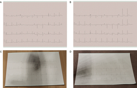
For each PTB-XL ECG, an image was created according to recommendations outlined in the ‘AHA/ACCF/HRS Recommendations for the Standardisation and Interpretation of the ECG’ document,13 comprising a continuous ten second recording divided into three rows and four columns consisting of 2.5 s of data for each lead where column 1 represents leads I, II and II; column 2 represents aVR, aVL and aVF; column 3 represents V1, V2 and V3 and column 4 represents V4, V5 and V6. An additional rhythm strip containing 10 s of data (lead II) was included for rhythm analysis.
The Blender (Blender Foundation, Amsterdam, Netherlands) software platform was used to create synthetic ECG images using custom code (developed by AB). ECG images were recreated by sampling 2.5 s epochs for each lead, positioned according to AHA/ACCF/HRS recommendations13 and with lead markers, lead labels and calibration scales added. Resulting waveform traces were superimposed onto a paper grid (with a resolution set to 150 Hz (25 mm/s) horizontally and 10.0 mm/mV vertically) leading to the generation of a single layout for each PTB-XL ECG. The resolution of the waveform image was set to 5 pixels/mm with a final image output size of 1397×1029 pixels for a 10 s trace.
To validate the accuracy of initial ECG images created from signal data, ECG files representing sine waves of known amplitude (0.5 mV) and frequency (1.25 Hz) were created using the WFDB Toolbox for MATLAB/Octave.14 A total of 12 test ECGs were created, consisting of ECGs with the sine wave at a single ECG lead location with all other leads set to a constant electrical potential of 0 mV. These files were converted into ECG images using the same code used for ECG recreation. All validation ECGs were inspected to confirm the correct location of the ECG leads. For each lead of each ECG containing a sine wave, the amplitude and cycle length (frequency) were measured by an observer (NB) blinded to the original amplitude and frequency. Spearman’s correlation coefficient was used to examine the correlation between measured and actual sine wave frequency and amplitude.
Creation of synthetic ECG images
To apply degradation techniques to ECG images (ie, to make it appear as though images had been photographed), ECGs were passed to a second render which placed each image trace on a 3D model comprising a paper sheet positioned in a synthetically developed workspace. In total, 352 unique geometric variations were created from 8 paper sheet variations, 11 workspaces and 4 synthetic workspace orientations. The Blender platform’s bpy module was used to create an automated Python script for ECG image generation. For each ECG, a mesh and synthetic workspace were randomly selected, and the location and rotation of the ECG paper sheet, camera and light sources were randomly adjusted. To mimic the imperfections associated with photographed ECGs, varying degrees of stucci noise were applied.15 This technique, which simulates the appearance of stucco (a wall structure containing holes and bumps), was chosen following a review of the imperfections encountered with real-world ECG photographs by a senior 3D technical artist (AB). For each image, the size and turbulence of the noise were randomly selected to introduce varying degrees of texture distortion.
Clinical Turing tests
A series of visual Turing tests were designed and conducted to assess the fidelity of synthetic ECG images via an online survey (Qualtrics, Provo, Utah, USA). In all rounds of Turing tests, healthcare professionals were provided with a series of 60 images comprising 30 synthetically created ECGs and 30 photographs of real-world ECGs. ECG images were redacted in areas where text may appear. Images were displayed one-by-one to participants and shown in uniform order. Participants were asked to select whether they thought the images were real or synthetic and, in the second and third rounds, to rate their confidence using a 5-point Likert scale (online supplemental figure S2). At the end of each survey, healthcare professionals were asked to provide qualitative feedback through a series of open questions. Feedback was summarised and used to iteratively improve the dataset’s fidelity. All readers decided whether each image was real or synthetic without any time limit and no prior knowledge regarding the number of real or synthetic images. To avoid bias, healthcare professionals were only allowed to complete one round of clinical Turing tests.
For each round of Turing tests, we measured the accuracy (overall proportion of ECGs correctly identified as ‘real-world’ or ‘synthetic’), true recognition rate (proportion of real-world ECGs identified correctly) and false recognition rate (proportion of synthetic ECGs identified correctly) using adapted terminology from previous Turing tests.16 17 The Fleiss-Kappa score was calculated to evaluate the degree of interobserver agreement. For the second and third rounds of clinical Turing tests, confidence Likert scale scores were converted to a signed ordinal scale for area under the curve-receiver operating characteristic (AUC-ROC) score analysis. The data were analysed using SPSS V.29 (IBM).
Quantitative similarity analysis of real-world and synthetic ECG images
The Fréchet Inception Distance,18 a metric which quantifies the similarity between real and synthetic images by comparing the statistical distributions of deep feature representations extracted from a pretrained InceptionV3 neural network, was used to assess the similarity between synthetic and real-world ECG images. The 30 real-world ECGs used for the final round of Turing tests were compared with two sets of synthetic ECG images derived from 30 PTB-XL files: (1) the 30 ECG images from the final round of Turing tests that contained visual imperfections and (2) the 30 corresponding synthetic ECG images without visual imperfections. Fréchet Inception Distance scores were calculated for both sets of images, with lower scores indicating greater similarity to the real-world ECG images. An unpaired t-test was performed to assess the difference in Fréchet Inception Distance scores.
Assessment of pre-existing image-based algorithms
To examine the performance of currently available image-based algorithms on the GenECG dataset, synthetic images were inputted into two image-based AI-ECG algorithms.11 19
The first image-based algorithm tested was ECG-Dx (https://www.cards-lab.org/ecgdx), an automated diagnostic algorithm capable of detecting six diagnoses (atrial fibrillation, sinus tachycardia, sinus bradycardia, left bundle branch block, right bundle branch block and first-degree atrioventricular block). We searched the PTB-XL database for these diagnoses and randomly selected 75 abnormal ECGs. Images with and without image degradation techniques were inputted into the web-based platform. The corresponding classifiers were compared with labels assigned from the PTB-XL dataset.
The second image-based algorithm examined was developed by Bridge et al, to distinguish ‘normal’ from ‘abnormal’ ECGs, and this algorithm has demonstrated good performance on scanned ECG printouts.19 This model was originally developed using 1172 ECGs and built on InceptionV3,20 a pretrained convolutional neural network, with extra layers added to improve performance and prevent overfitting. Due to the unavailability of the original model weights and ECG dataset, we trained an identical model using 1682 images from the ‘ECG images dataset of Cardiac and COVID-19 patients,’ an open-access dataset.10 The dataset contains five distinct categories: COVID-19 (n=250), myocardial infarction (n=74), abnormal heart beat (n=546), history of myocardial infarction (n=203) and normal person ECG images (n=859). Given the anticipated challenges in distinguishing normal versus abnormal ECGs in COVID-19 patients, we excluded images from the COVID-19 category. The remaining 1682 images were defined as normal (n=859) or abnormal (n=823), and randomly split into train (n=1082), validation (n=200) and test datasets (n=400).
To assess the algorithm’s ability to analyse synthetic data, we searched the PTB-XL dataset for ECGs which the algorithm would class as either ‘normal’ or ‘abnormal’ and randomly selected 215 GenECG images (96 normal, 119 abnormal) containing image degradation techniques. The images were randomly split into train (n=150), validation (n=22) and test (n=43) images. The trained model was applied to evaluate its performance on the 43 test synthetic ECG images. Following the initial results, the model had low efficiency on synthetic GenECG images since it was not exposed to images that resembled our images during training. Therefore, the model was fine-tuned on the train and validation images (n=172) using weights from the model trained on the open-access dataset as initial weights. The additional layers of the Bridge et al model were adjusted accordingly.
To assess the generalisation power of the synthetic model and to ensure that the model did not over-fit during fine-tuning, we re-evaluated the trained synthetic model over the 400 test dataset images derived from the ‘ECG images dataset of Cardiac and COVID-19 patients’ dataset.10 Additionally, we evaluated the performance of both the initially developed model and the fine-tuned model on 79 real-world ECG images obtained using methodology described by Sangha et al.11 Images which would have been defined as either normal (n=24) or abnormal by the Bridge et al, algorithm (five abnormal ECGs for each label of interest: sinus arrhythmia, atrial fibrillation, atrial flutter, premature atrial contraction, premature ventricular contraction, atrioventricular block, ventricular tachycardia, supraventricular tachycardia, Wolff-Parkinson-White syndrome, paced rhythm, junctional rhythm)19 were obtained from both the life in the fast lane website (https://litfl.com/ecg-library/) and Google searches. The images contained visual imperfections typically encountered in routine clinical care.
ECG images were preprocessed by cropping the region of interest using the rembg Python library (https://pypi.org/project/rembg/2.0.28/) to remove the background of each image. Images were then resized using the Lanczos method to ensure uniform input into the image-based model.21 Subsequently, AUC-ROC analysis was performed to evaluate model performance.
[ad_2]
Source link